Improvements Getting Better at doing Deep Learning
Table of Contents:
Last week, we looked at some fundamental concepts in training deep neural networks. This week, we’ll expand on the idea by going deeper into important concepts such as regularization, weight init, adaptive optimizers and if time permits, learning rate schedules. That said, let’s get started.
The Tensorflow documentation is a excellent resource for all things TF/Keras and will be the source we’ll use for classifying images on the FMNIST dataset. Click here to go to a Google Colab notebook.
For PyTorch, a short notebook can be found here
That said, let’s dive in!
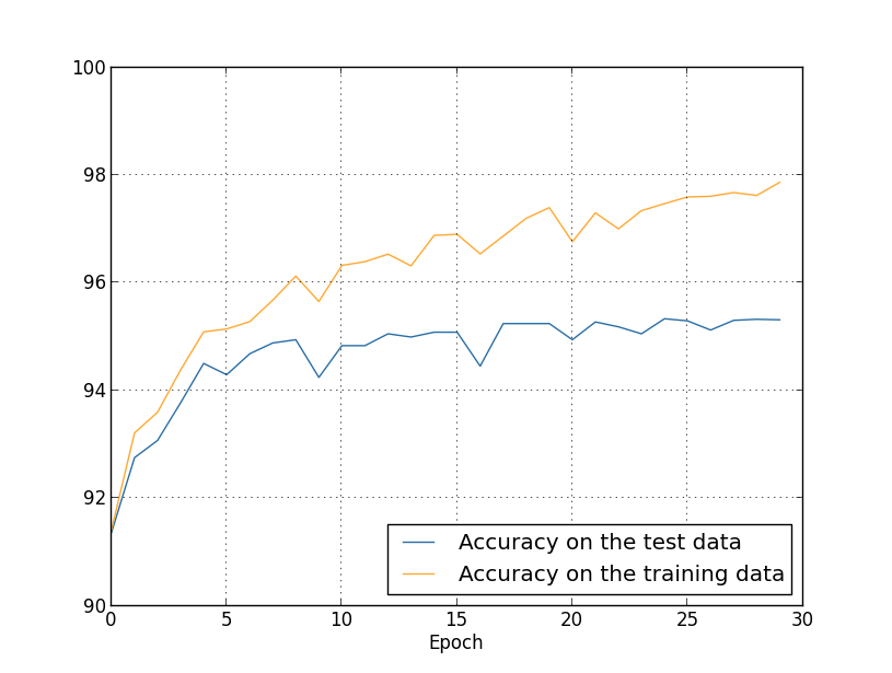
Dealing with overfitting
Deep neural networks are incredible flexible in terms of the data they can represent. The question to ask is, are these networks powerful because of the freedom such a large space allows in terms of representing data or are they actually learning some meaningful insights from the data they’re trained on?
In most cases, it is plausible to assume that the network is actually overfitting on the training data rather than learning the inherent distributions and any meaningful patterns contained within the data.
Overfitting, in terms of metrics, occurs when the accuracy for the test set is not in line with the train set. Of course, it’s much more nuanced than that, but this is the working definition for us. What that means is the network we train is learning the data and noise specific to the train set rather than learning about the distribution space that the training data is drawn from.
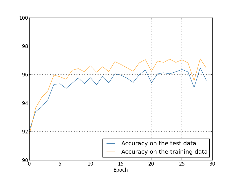
The first approach we’ll look at for dealing with overfitting is called early stopping. We’ll use the validation set as an abstraction layer here. For every loop through our data, we’ll look at our validation accuracy and once it stops getting better, we stop training further. In reality, we’ll just go back to the state of the network at that instant rather than stop training. This is how Keras implements early stopping, as a callback function that you can add to your model which continuously monitors the accuracy and saves the state(weights, bias and hyperparams) at the epoch.
Next, let’s look at regularization, which lets us deal with overfitting on ever-increasing architecture sizes.
L2 Regularization
Also known as Ridge Regularization, L2 will add a regularization term that’s the sum of the square of all the weights in the network. This regularization term is scaled by a factor of λ/2n.
Mathematically, it is represented as where C0 is the original cost function.
Simply put, L2 will force the weights to be small, with the idea being that small weights won’t lead to large deviations from the expected path. λ controls what term in the cost function gets more importance and the larger the value of λ the more preference is given to smaller weights.
From a gradient descent perspective, the learning rate will end up being scaled by a factor of . This factor is also called as weight decay, and does exactly what you think. The weights are being driven towards zero, controlled by the regularization coefficient λ.
But why and how does L2 actually work?
During backpropagation, the learning rule adds a weight delta value to each weight. This weight delta is basically a fraction of the derivative of the error function. This is all multiplied by the learning rule hyperparameter. If you take the derivative of the regularization term, the exponent 2 and the divide by half-term cancel out leaving the update rule to be λ * w. This essentially puts us in control of the penalty we give to the network for larger weigthts. Smaller weights won’t change the behaviour of the network too much, instead learning to recognize patterns that are evident throughout the network rather than local noise.
Before L2
After L2
L1 Regularization
L1 regularization is intuitively similar to L2, except now we add the sum of the absolute values of the weights rather than the sum of squares.
Mathematically, it is represented as
In L2, weight decay is proportional to w whereas weight deacy in L1 is by a constant amount. For large weights, L1 shrinks the weight much less than L2 and vice versa. This leads to L1 weights being sparse, with a majority of the weights driven to 0 while some of them turn up to 1.
We’ve covered a lot of ground in the last week or so. Starting with loss functions, activation functions to regularization and overfitting strategies such as dropout, we’ve come a long way. Let’s tackle two more fundamental pieces before we move onto the cool stuff.
Weight Initialization strategies
Weight initialization is a very powerful yet simple technique that can be the difference between a network converging in a couple of hours(very ad-hoc I know!) versus say, a couple hundred iterations. The only thing that a neural network does is update weights and bias vectors using the gradient descent learning rule. However, it does at a scale of roughly millions of weights and biases parameters which makes weight initialization such an effective and important strategy.
Let’s jump into Xavier initialization and we’ll cycle back to why and what later.
Xavier init lets us initialize weights such that variance is the same for the input and the target. We want to start out with values that are not too small or too large, trying to ensure that they don’t end up in the saturated region of the activation function we’ll choose to use.
Rather than using random initialization following a normalized Gaussian distribution(std dev of 1 and mean of 0), we’ll initialize it with a Gaussian with mean 0 and std dev of , squashing down the Gaussian by a factor of √. The idea is not to avoid Gaussian distributions, but to avoid falling in the trap of saturated weights that contribute nothing to training. This is again, highly superficial and there’s a fair amount of math that deals with using √. For an overview, and extension to Kaiming ReLu initialization, check out this blog.